Accretion discs/3. Analytic models of accretion discs

From Scholarpedia

This article has not been published yet; It may be unfinished, contain inaccuracies or unapproved changes.

Author: Dr. Marek A. Abramowicz, Physics Department, Göteborg University, Sweden and N. Copernicus Astronomical Center, PAN, Warsaw, Poland
Author: Miss Odele Straub, N. Copernicus Astronomical Center PAN, Warsaw, Poland

Analytic models describe extreme geometries, matter supplies and optical depths

Non-linear, coupled partial differential equations of radiative viscous hydrodynamics (or magnetohydrodynamics) that describe physics of accretion discs are too complex to be exactly solved analytically in the general case. Usually, analytic models assume that the accretion is stationary and axially symmetric. For such discs, useful approximate solutions exist in extreme cases corresponding to the following three fundamental divisions (as shown in Figure 1):

Geometry: vertically "thin" versus "thick" discs

Mass supply rate: "sub" versus "super" Eddington accretion rate

Optical depth: "opaque" versus "transparent" discs

Subsection 3.1. Thin discs covers accretion disc models with H/R < 1 that includes Shakura-Sunyaev, slim and adafs.
Subsection 3.2. Thick discs covers accretion disc models with H/R > 1 that includes Polish doughnuts and ion tori.

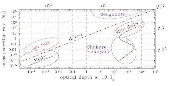
The main types of analytic accretion disc models in the parameter space of different geometries (i.e. vertical thickness), matter supplies (i.e. accretion rates) and optical depths. Credit: Aleksander Sadowski (2009)

Extreme geometries: vertically "thin" and "thick" accretion discs

A thin discs has its "vertical" (i.e. across the disk plane) extension much smaller than its "radial" (along the plane) extension, $H \ll R$ . This means that the disc structure depends mostly on the radial coordinate $R$ and may be described by ordinary differential equations. Thick discs have toroidal shapes with $H \approx R$ . In this case, the analytic solution is possible because simplifying assumptions concerning mostly physics. Detailed models of thin and thick discs are described in the sub-sections of this Scholarpedia article: 3.1. Thin discs, 3.2. Thick discs.

Extreme mass supply : "sub" and "super" Eddington accretion rates

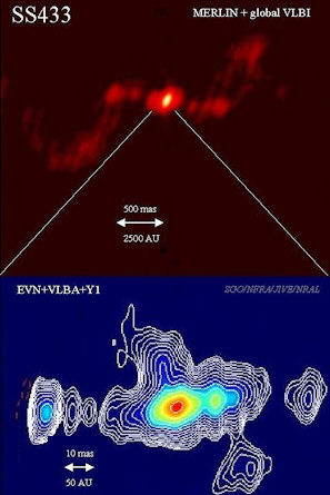
Radio maps of SS433, a source containing a super-Eddington accretion disc. SS433 may be a Galactic prototype of the ultraluminous X-ray sources (ULXs) found in other galaxies.

The accretion rate is defined as the instantaneous mass flux through a spherical surface $r =\,\,$ const inside the disc. In non-stationary accretion discs accretion rate depends on both time and location, but in stationary disc models with no substantial outflows (no strong winds) it is

${\dot M}(r, t) = const.$

Accretion discs may be divided into two classes, depending on whether accretion rate is much smaller than, or comparable to the characteristic Eddington accretion rate, that depends only on the mass of the central accreting object $M$ ,

${\dot M}_{Edd} = {L_{Edd}/c^2} =1.5 \times 10^{17}\,({M /M_0})\,[{\rm g}/{\rm sec}].$

Here $M_0 = 2 \times 10^{33}\,$ [g] denotes the mass of the Sun, and $L_{Edd}$ is the Eddington luminosity (radiation power), familiar from the theory of stellar equilibria: at the surface of a star shining at the Eddington rate, the radiation pressure force balances the gravity force.

Figure on the left shows radio maps of SS433, a well-known Galactic object with a super-Eddington accretion disc.

A rather common belief that a black hole cannot accrete at a rate higher than the Eddington one is wrong. In particular, the Eddington rate is not a limit for the mass growth rate of a black hole due to accretion, $dM/dt$ . It could be that $dM/dt \gg {\dot M}_{Edd}$ . This is relevant for modeling the cosmological evolution of black holes.

M.A. Abramowicz, Super-Eddington black hole accretion: Polish doughnuts and slim disks

A.R. King, Hyperaccretion

Extreme optical depth: "opaque" and "transparent" accretion discs

Note: a more detailed discussion of the subject presented in this Section is given in Narayan & Yi,1995, ApJ, 452,710. Optical depth in vertical direction $Z$ is approximated by $\tau = \Sigma \kappa H$ . Here $\kappa$ is the opacity coefficient, and $\Sigma$ is the surface density, i.e. vertically integrated density.

Opaque discs ( $\tau \gg 1$ ): Such discs are not very hot, the temperature is much less than the virial temperature, $T \ll T_{vir} = ????$ . Simple (and often used) analytic models approximate the flux emitted locally (at a fixed radius $R$ ) from the disk surface by the "diffusive" black body formula, $f = f(R) = {8\sigma T^4}/{3H\tau}$ . In calculating spectra, the total flux from whole surface of accretion disc is (roughly) approximated by the Planck formula,

$F_{\nu}=4\pi \frac{\nu^3 \cos i}{c^2 d^2}\int^{R_{out}}_{R_{in}}\frac{R}{\exp[h\nu/kT(R)]-1}dR,$

where $d$ and $i$ are the distance and inclination angle to the rotation axis, respectively, as seen by an observer. More advanced models solve (approximately) radiative transfer equation in the vertical direction (see e.g. REFERENCES SHOULD BE ADDED), considering dependence on the radiation frequency $\nu$ .

Transparent discs ( $\tau \ll 1$ ): Such discs have relatively high-temperatures and low-densities. Bremsstrahlung, synchrorton and Copmton radiative processes are most relevant, $f = f_{br} + f_{br,C} + f_{syn} + f_{syn,C}$ . They cool down the electrons in the gas much more efficiently than the ions, and therefore a temperature separation between electrons $T_e$ and ions $T_i$ is expected. Radiative cooling by Bremsstrahlung, $f^-_{br} = f_{ei} + f_{ee}$ is given by,

$f_{ei} = n_e n_i c \sigma_T \alpha_f m_e c^2 F_{ei}(\theta_e) \,\, [{\rm erg \,\, cm^{-3} \,\, s^{-1}}],$ where $F_{ei}(\theta_e<1) = 4 (\frac{2 \theta_e}{\pi^3})^{1/2} (1 + 1.781 \theta_e^{1.34})$ and $F_{ei}(\theta_e>1) = \frac{9 \theta_e}{2\pi}[\ln(1.123 \theta_e + 0.48) + 1.5]$

$f_{ee} = n_e^2 c r_e^2 \alpha_f m_e c^2 F_{ee}(\theta_e) \,\, [{\rm erg \,\, cm^{-3} \,\, s^{-1}}],$ where $F_{ee}(\theta_e<1) = \frac{20}{9 \pi^{1/2}}(44-3\pi^2)\theta_e^{3/2} (1+1.1\theta_e^2 - 1.25\theta_e^{5/2})$ and $F_{ee}(\theta_e>1) = 24 \theta_e [\ln(0.5616 \theta_e) + 1.28]$

$f_{br,C} = 3\eta_1\{\frac{1}{3}(1-\frac{x_c}{\theta_e})-\frac{1}{\eta_3+1}[(\frac{1}{3})^{\eta_3+1}-(\frac{1}{3\theta_e})^{\eta_3+1}]\} f_{br},$

where $n_e$ and $n_i$ are the number densities of electrons and ions, $\sigma_T$ is the Thomson cross-section and $\alpha_f$ the fine structure constant, $m_e$ and $r_e = e^2/m_ec^2$ are the electron's mass and radius and $c$ the speed of light. $F_{ee}(\theta_e)$ and $F_{ei}(\theta_e)$ are the radiation rate functions, given by the dimensionless electron temperature $\theta_e = kT_e/m_ec^2$ . The Compton enhancement factor $\eta = \eta_1 + \eta_2 + ({x}/{\theta_e})^{\eta_3}$ is given by $\eta_1 = P(A-1)/(1-PA)$ , $\eta_1 = -3^{-\eta_3} \eta_1$ and $\eta_3 = - 1 - \ln P / \ln A$ , where $x = h\nu/m_ec^2$ , factor $P$ is the probability that a photon scatters and $A$ is the mean energy amplification factor by that photon and $x_c = h\nu_c/m_e c^2$ . If a magnetic field $B$ is present, there is also radiative cooling by synchrotron emission:

$f_{syn} = \frac{2\pi}{3c^2}kT_e(R)\frac{d\nu_c^3(R)}{dR}\,, ~~f_{syn,C} = [\eta_1 - \eta_2(\frac{x_c}{\theta_e})^{\eta_3}] f_{syn}\,, ~~ \nu_c = \frac{3 e B}{4 \pi m_e c} \theta_e^2 x_M,$

where the coefficient $x_M$ must be numerically calculated from a relativistic Maxwellian distribution of electrons.

> PREVIOUS SECTION 2.1. The black hole gravity

> FIRST SECTION Scholarpedia Accretion discs

> NEXT SECTION 3.1. Thin discs

Invited by:

Eugene M. Izhikevich

Accretion discs/3. Analytic models of accretion discs

From Scholarpedia

Contents

Analytic models describe extreme geometries, matter supplies and optical depths

Extreme geometries: vertically "thin" and "thick" accretion discs

Extreme mass supply : "sub" and "super" Eddington accretion rates

Extreme optical depth: "opaque" and "transparent" accretion discs

Views

Personal tools

Scholarpedia

Encyclopedia of

for readers

for authors

Toolbox